Performance Analysis

Chapter 18

Intro

Analysis of Algorithms

Dilemma: You have two (or more) methods to solve a problem.
How do you choose the BEST method?

• One approach: Implement each algorithm in C++; test how long each takes to run.

• Problems:

  • Different implementations may cause an algorithm to run faster/slower.

  • Some algorithms run faster on some computers.

  • Algorithms may perform differently depending on data (e.g., sorting often depends on what is being sorted).

A Fundamental Computer Science Challenge

• One of the most fundamental tools for computer scientists to analyze the cost of an algorithm.

• The cost can be described in terms of time, space (memory usage), electricity, etc.

• Ideally, we will develop a simple scheme to rank algorithms from best to worst.

Approaches to Analyzing Performance

Comment on the “general” performance of the algorithm using one of two options:

1. Empirical: Measure performance for several examples.
   But, what does this tell us in general?

2. Analytical:

   • Instead, assess performance in an abstract, generalized manner.

   • Idea: analyze performance as the size of problem growth.

   • Examples:

     • Sorting: How many comparisons for an array of size ?

     • Searching: How many comparisons for an array of size ?

   • Challenge: It may be difficult to discover a reasonable formula.

Analytical Approach: Step 1 of 2

Characterize performance by counting the number of of key operations.

• For a sorting algorithm, the key operations includes
  the number of times:

  • two values are compared and

  • two values are swapped.

• Search:

  • Count the number of times the value being searched for is compared to values in an array.

• Recursive function:

  • Count the number of recursive calls.

Analysis with Varying Results

• Example: some sorting algorithms may require as few as comparisons and as many as .

• Types of analyses based a problem of size :

  • Best case: What is the shortest an algorithm can run?

  • Average case: On average, how fast does an algorithm run?

  • Worst case: What is the longest an algorithm can run?

• Computer scientists usually use worst-case or average-case analysis.

  • What are some example domains where you may care more about the worst case than the average case and vice versa?

Notice: We Are Estimating

• Usually, we approximate or estimate the performance of an algorithm, assuming it is operating on a very large data set.

• Estimation is an important skill to learn and use.

Simpler Question: How many hotdogs tall is the Empire State Building?

• The ESB is feet tall.

• Assuming that a hotdog is 6 inches from end to end, you would need, hotdogs.

The Empire State Building

Complexity Analysis

Analysis

• An objective way to evaluate the cost of an algorithm or code section.

• The cost is usually computed in terms of time or space.

• The goal is to have a meaningful way to compare algorithms based on a common measure.

Algorithm Analysis

• Algorithm analysis requires a set of rules to determine how operations are to be counted.

• There is no generally accepted set of rules for algorithm analysis.

• In some cases, an exact count of operations is desired; in other cases, a general approximation is sufficient.

• The following rules are typical of those intended to exactly count operations.

Rules for Estimation

1. We assume an arbitrary time unit.

2. Execution of one of the following operations takes time 1:

   • assignment operation

   • single I/O operations

   • single Boolean operations, numeric comparisons

   • single arithmetic operations

   • function return

   • array index operations, pointer dereferences

Example 1

count = count + 1;  // Cost: c₁
sum = sum + count;  // Cost: c₂

Total Cost = .
Because we assume the addition costs 1 and assignment costs 1, the total cost is 4 units.

Conditional Cost

if (n < 0) {     // Cost: c₁ = 1$
    absVal = -n; // Cost: c₂ = 2$
} else {
    absVal = n;  // Cost: c₃ = 1$
}

• is the cost of the boolean evaluation ( instruction).

• is the cost of the negating a number () + the cost of assignment ().

• is the cost of an assignment ().

• Worse Case	Best Cast	Average

Example 3

i = 1;             // Cost: c₁ = 1
sum = 0;           // Cost: c₂ = 1
while (i <= n) {   // Cost: c₃ = 1
    i = i + 1;     // Cost: c₄ = 1 + 1 = 2
    sum = sum + i; // Cost: c₅ = 2
}

• Remember assignment (=) and addition (+) each cost .

• How many times does the loop execute?
  times.

• 
  

More Rules for Estimation

3. Selection statement (if, switch) time is the time for the condition evaluation, plus the maximum of the running times for the individual clauses in the selection.

4. Loop execution time is the number or iterations multiplied by its body’s execution time, plus the time for the loop check and update operations, plus the loop setup time.
   Always assume that the loop iterates the maximum number of times.

5. The runtime of a function call is 1 for setup plus the time for any parameter calculations plus the time required for the execution of the function body.

Nested Example

i = 1;                 // c₁ = 1
sum = 0;               // c₂ = 1
while (i <= n) {       // c₃ = 1
    j = 1;             // c₄ = 1
    while (j <= n) {   // c₅ = 1
        sum += i;      // c₆ = 2
        ++j;           // c₇ = 2
    }
    ++i;               // c₈ = 2
}

• The outer loop iterates times.

• For each iteration of the outer loop, the inner loop iterates times.

• The total cost is:

Important Note: is the highest (largest) term!

Big O Notation

Comparing Algorithms

• An algorithm’s time requirement is a function of the problem size.

• The problem size depends on the application (e.g., the number of list elements for a sorting algorithm).

• For instance, we say that (if the problem size is )

  • Algorithm A requires time units to solve a problem of size .

  • Algorithm B requires time units to solve a problem of size .

  

  Comparing Algorithm A () with Algorithm B ()

  

  Comparing Algorithm A () with Algorithm B ()

Comparing Algorithms

• An algorithm’s proportional time requirement is known as the growth rate.

• We can compare the efficiency of algorithms by comparing their growth rates.

Comparing Algorithms

Example: Which is faster?

It depends on .

1	120	37
2	511	71
3	1,374	159
4	2,895	397
5	5,260	1,073
6	8,655	3,051
7	13,266	8,923
8	19,279	26,465
9	26,880	79,005
10	36,255	236,527

One term dominated the others.

We only care about the highest-order (dominating) term.

1	37	32.4%
2	71	50.7%
3	159	67.9%
4	397	81.6%
5	1,073	90.6%
⋮	⋮	⋮
9	79,005	99.7%
10	236,527	99.9%

As Grows, Some Terms Dominate

	n=10	n=100	n=1,000	n=10,000	n=100,000
or
			...

Asymptotic growth rates of common complexity functions, from logarithmic to factorial, illustrating their relative scaling for increasing .

Asymptotic growth rates of common complexity functions, from logarithmic to factorial, illustrating their relative scaling for increasing

Big

• If Algorithm A requires time proportional to ,
  Algorithm A is said to be order , and it is denoted as .

• The function is called the algorithm’s growth-rate function.

• Since the capital is used in the notation, this notation is called the Big- notation.

• If Algorithm A requires time proportional to , it is .

• If Algorithm A requires time proportional to , it is .

Example 1

• If an algorithm requires seconds to solve a problem size, .

• If constants and exist such that
  for all and ,
  then the algorithm is order . (In fact, is 3 and is 2)

• Thus, the algorithm requires no more than time units.

• So it is

More Examples

This game of “spot the highest term” is actually not difficult!

• =

• =

It can get somewhat tricky:

• =

• =

Growth Rate Functions Generalized

Big O	Time requirement as problem size increase
	Constant is independent of the problem’s size.
	Logarithmic increases increases slowly.
	Linear increases directly.
	Increases more rapidly than linear algorithms.
	Quadratic increases rapidly.
	Cubic increases more rapidly than a quadratic algorithm.
	Exponential is impractical.

Practice

Example 1:

i = 1;           // Cost: c₁
sum = 0;         // Cost: c₂
while (i <= n) { // Cost: c₃
    ++i;         // Cost: c₄
    sum += i;    // Cost: c₅
}

Example 2:

i = 1;               // Cost: c₁
sum = 0;             // Cost: c₂
while (i <= n) {     // Cost: c₃
    j = 1;           // Cost: c₄
    while (j <= n) { // Cost: c₅
        sum += i;    // Cost: c₆
        ++j;         // Cost: c₇
    }
    ++i;             // Cost: c₈
}

Example 3:

for (i = 1; i <= n; i++) {         // Cost: c₁
    for (j = 1; j <= i; j++) {     // Cost: c₂
        for (k = 1; k <= j; k++) { // Cost: c₃
            ++x;                   // Cost: c₄ = 2$
        }
    }
}

Notice: We do NOT need to know the exact number of iterations to find the Big-.

Example 4: Recursion can be hard.

The Tower of Hanoi is a puzzle consisting of three rods some disks of different diameters, which can slide onto any rod. The goal is to move the disc to a different rode. However, a larger disk cannot be placed on top of a smaller one.

Tower of Hanoi

Example Solution

void hanoi(int n, char source, char dest, char spare) { // Function-call cost
  if (n > 0) {                                     // Cost: c₁
    hanoi(n-1, source, spare, dest);               // Cost: c₂
    cout << "Move top disk from pole " << source
      << " to pole " << dest << endl;              // Cost: c₃
    hanoi(n-1, spare, dest, source);               // Cost: c₄
  }
}

• By now, I hope you see that constant and coefficient costs are virtually superfluous when working with Big .

• To find the growth-rate function for a recursive algorithm, we have to solve its recurrence relation.

• You will learn how to do this in Discrete Math.

What is the cost of hanoi(n, 'A', 'B', 'C')?

• When ,

• When ,
  =
  = recurrence equation for the growth-rate function of hanoi-towers algorithm.

• Now, we have to solve this recurrence equation to find the growth-rate function of the hanoi-towers algorithm.

• This turns out to be because for every we make calls.

Example 5:

int bigOExample5(int n)
{
  int res = 0;
  int m = 4 * n;
  int *pArray = new int[m] {};

  for(int i = 0; i < m; i++) {
    m_pArray[i] = i;
  }

  for(int i = 0; i < m; i++) {
    res += m_pArray[i];
  }

  delete[] pArray;

  return res;
}

Example 6:

int bigOExample6(int n)
{
  int total = 0;

  for(int i = 0; i < 4 * n; i++)
  {
    total += i;
  
    for(int j = 0; j < 4; j++)
    {
      total += j;
    }
  }

  return total;
}

Example 7:

int bigOExample7(int n) {
  int total = 0;
  for(int i = 0; i < n; i++) {
    for(int j = 1; j <= n; j *= 2) {
      total += j;
    }
  }

  return total;
}

Measuring Time

Empirical Measurement

• While analytical performance measures are important, an empirical approach is also insightful.

• The naive way to take timings:

  1. Record the start time.

  2. Run section of code you wish to time.

  3. Record the end time.

  4. Your answer is (end – start).

• While there are numerous issues with this approach, it will give sufficient approximate timings for this class.

Template Code for Timing a Function

#include <iostream> // To display information
#include <chrono>   // Required for taking timings

void checkTime(const unsigned int MIN_N, const unsigned int MAX_N, const unsigned int CHANGE_IN_N) {
  using namespace std::chrono;

  // We want to run our algorithm over varying sizes.
  for (unsigned int size = MIN_N; size < MAX_N; size += CHANGE_IN_N) {
    // Capture the start clock (stored as clock_t)
    const auto START_TIME = (high_resolution_clock::now());

    // To Do: This is were your algorithm should be called.
    // Note: size is the SIZE or the input; you may have to change it.
    // functionCallToYouAlgorithm(size);

    // Capture the clock and subtract the start to get the total time elapsed.
    const auto DIFF = duration_cast<microseconds>(high_resolution_clock::now() - START_TIME);

    // Convert clock_t into seconds as a floating point number.
    const auto TIME_AMOUNT = static_cast<double>(DIFF.count()) * 1e-6;

    // Print out first the size (size) and then the elapsed time.
    std::cout << size << '\t' << TIME_AMOUNT << '\n';
  }
}

Example Output

First is the size (1000) and second is the number of seconds (pretty small).

1000  4e-06
2000  8e-06
3000  1.2e-05
4000  2.5e-05
5000  2.9e-05
6000  2.4e-05
7000  3.5e-05
8000  2.9e-05
9000  3.2e-05
10000 3.5e-05
11000 3.9e-05
12000 4.2e-05
13000 4.5e-05
14000 5.2e-05
15000 5.6e-05
16000 6e-05
17000 6.5e-05
18000 6.8e-05
19000 7e-05
20000 7.6e-05

Gnuplot

Crash Course in gnuplot

gnuplot is an interactive plotting program.

• To install, type:

  sudo apt update && sudo apt install gnuplot -y

• To run, type: gnuplot

Example Plot: A Higher-Order Knot in gnuplot

Example Plot: A Higher-Order Knot in gnuplot

Basic Example

Try typing the following commands:

• Open gnuplot: gnuplot

• Display a sin wave: plot sin(x) with line

  

  gnuplot of sin(x)

• Change from a line to points: plot sin(x) with point

  

  gnuplot of sin(x) with points

Add Labels to the Plot

Type the following to label your plot.

set title "Sin Wave"           # Add a title to the top.
set ylabel "Amplitude"         # Label the y axis.
set xlabel "Time (in Seconds)" # Label the x axis.
replot                         # Show these changes.

gnuplot of sin(x) with title and labels

Save a Plot to File

To output the plot to a PDF instead of the screen:

set terminal pdf color
set output "nameofplot.pdf"

• Then type the commands to plot your data.

• To save an already-created plot, add replot or rep to re-plot it in the new output (PDF) device.

• The data will be written when you exit gnuplot.
  exit

To save the current plot to a file.

save "plotname.pdf"

Opening PDF files in Visual Studio Code

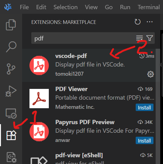
• For convince, I recommend installing a PDF viewer extension to Visual Studio Code like vscode-pdf.

• If you are using the Windows Subsystem for Linux (WSL), also install the WSL extension by Microsoft. After that, you should see a green box in the bottom left saying “WSL:Ubuntu”.

• The following examples assume you can open PDFs in Visual Studio Code.

Huge Time Saver!

gnuplot commands can be saved to a script file and automatically used.

• Create a file named simple.plot containing the following:

  set terminal pdf color
  set output "simple.pdf"
  set ylabel "Time (seconds)"
  set xlabel "Size"
  
  # Add additional commands to create the plot...

• Run your script and display the PDF: gnuplot simple.plot && code simple.pdf

Huge Time Saver!

Using a gnuplot script is especially useful if you put it in a makefile!

plot:
  gnuplot simple.plot # Run gnuplot script
  code simple.pdf # Open the PDF is Visual Studio Code

Now, make plot generates the plot and displays it!

Plotting Timings

Plotting

• Assume we have the full listing of performance
  data in a file named single-timings.data.

• With gnuplot, we can simply graph the timings:
  plot "single-timings.data" using 1:2 with line

  

  Plotting Timing Data

  set terminal pdf color
  set output "single-timings.data"    # Name the output file
  
  set title "Algorithm Performance"
  set ylabel "Time (in seconds)"
  set xlabel "Data Size"
  set grid # Show grid lines
  
  # Make line thicker with lw 3
  # Change the line's title with title "Runtime"
  plot "single-timings.data" using 1:2 with line lw 3 title "Runtime"

Automate Testings with a Makefile

.PHONY: plot
all: data.pdf

main: timing-example.cpp
  g++ -Wall -Wextra timing-example.cpp -o main

data.out: main
  ./main > data.out

data.pdf: data.out data.plot
  gnuplot data.plot
  code data.pdf # Open PDF in VS Code (extension required)

plot: data.pdf

Plotting Multiple Lines from Multiple Files

Let us assume we have two files (in the same format), each with timing data for a different algorithm.

• With gnuplot, we can graph both timings:

  plot "sumOfOneTo.data" using 1:2 with line, \
    "intersectionCount.data" using 1:2 with line

  

  Plotting Multiple Lines on One Graph

• You can append more and more data files in this manner.

Common Gotcha

• You only see one of the two algorithms you plotted!

  plot "linear1.data" using 1:2 with line lw 4 title "Linear Algorithm",\
    "quad2.data" using 1:2 with line lw 4 title "Quadratic Algorithm"

  

• Check your data and axis. Often it is too small to see.

  # Manually set the upper limit of the y-axis to 2
  plot [:][:0.0001] \
    "linear1.data" using 1:2 with line lw 4 title "Linear Algorithm",\
    "quad2.data" using 1:2 with line lw 4 title "Quadratic Algorithm"

  

Summary

• In review, we can:

  • Analyze an algorithm analytically to predict performance.

  • Profile programs to find what piece of code is the bottleneck.

  • Output & plot timings to see actual performance.

• We can spend many hours on performance analysis.

• We stick with the basics for this class.

Performance Tips

• Optimize the correct functions and look for the correct improvements.

• From our example, pref gives the following:
  

• Most of the time is spent in sumOfOneTo(); improving sumOfOneTo()’s performance may help.

• Optimizing sumOfOneToSquared() will not help as much.

  • Maybe we can memoize past results to use in the future
    or use a better data structure.

Summary

• We are scratching the surface.

• Important outcomes. You should be able to:

  • Analytically deduce the performance of code.

  • Profile code to find the hot spots.

  • Empirically run programs to evaluate performance.

  • Understand that some anomalies will not be addressed in this course.

Lab 7: Performance Analysis

Let’s take a look at Lab 7.